Quantile-based categorical statistics

Johannes Jenkner, Institute for Atmospheric and Climate Science, ETH Zurich, Switzerland

Traditional point-to-point verification is more and more superseded by situation-based verification such as an object-oriented mode. One main reason is that difficulties are encountered while interpreting the outcome of a conventional contingency table based on amplitude thresholds. Firstly, a predetermined amplitude threshold splits the distributions under comparison at an unknown location. In an extreme case, single entries of the contingency table can become zero. Then some scores cannot be computed (due to a division by zero) and statements about model behavior are hard to make. Secondly, the distributions under comparison usually differ considerably with respect to their range of values. Customary scores do not fulfill the requirements for equitability (Gandin and Murphy, 1992) and fail to be firm with respect to hedging (Stephenson, 2000). Thirdly, the joint distribution usually comprises multiple degrees of freedom. In the case of a 2x2 amplitude-based contingency table, three linearly independent scores are needed to display all verification aspects (Stephenson, 2000). It is possible to draw complementary information from the considered datasets, if concurrent scores are applied simultaneously. But it remains unclear, how to attribute individual verification aspects to measures which are not totally independent from each other. Fourthly, it is not meaningful to integrate amplitude-based scores over a range of intensities. Averages over multiple thresholds are difficult to interpret, because it is not obvious how many data points fall within individual ranges of thresholds.

To counteract the addressed drawbacks of categorical statistics, frequency thresholds, i.e. quantiles, can be used instead of amplitude thresholds to define the contingency table. Then two additional interrelations are automatically included into the conceptual formulation:

false alarms = misses misses + correct negatives = pN

Note that p denotes the quantile probability (0 < p < 1) and N stands for the sample size. Due to the first equation, the contingency table benefits from a calibration and is not influenced by the bias any more. The problem of hedging is eluded, because it is no longer possible to change the number of forecasted events without adjusting the number of observed events. Due to the second equation, the base rate (1–p) is fixed a priori and determines the rarity of events. The single remaining degree of freedom uniquely describes the joint distribution. Thus, it is now possible to describe the forecast accuracy or the skill related to individual intensities by means of a single score.

Depending on the quantile probability, the four entries of the contingency table only vary within a limited span (Fig. 1). If the quantile probability is below 0.5, there are always some hits by definition. If the quantile probability is above 0.5, there are always some correct negatives by definition. The misses and false alarms are consistently limited at the top. They are restricted either by the number of non-events (p < 0.5) or by the number of events (p > 0.5). A random forecast imposes strongly varying frequencies for all entries in the contingency table. A score is preferably independent from all variations caused by the base rate.

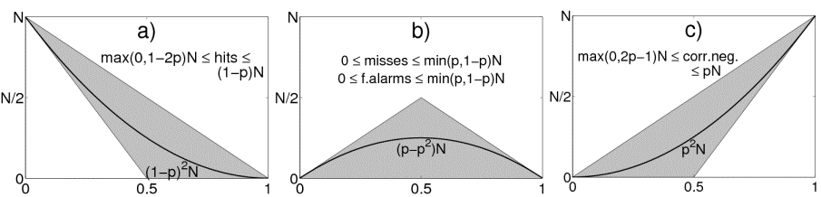
Figure 1: Possible entries (gray shaded) and random expectation values (thick black lines) of the four entries in the 2x2 contingency table: a) hits, b) misses or false alarms, c) correct negatives. The x-axis displays the range of quantile probabilities and the y-axis shows the number of data points.

The Peirce Skill Score (PSS, equivalent to the True Skill Statistics and the Hanssen-Kuipers Discriminant) is able to measure skill without being perturbed by the base rate (e.g. Woodcock, 1976, Mason, 1989). Thus, the PSS is ideally suited to measure the joint distribution, i.e. to display the forecast accuracy on its own. Owing to the definition of a quantile, the computation of the PSS simplifies to:

PSS = 1 – misses/misses_rand misses_rand = (p – p²)N

To complement the verification, the bias is represented by the absolute (abs) or relative (rel) quantile difference (QD):

QD_abs = q_mod – q_obs QD_rel = 2QD_abs/(q_obs + q_mod)

Note that q_obs and q_mod denote the observed and modeled (forecasted) quantile values, respectively. QD_rel is computed according to the amplitude component in the SAL measure (Wernli et.al., 2008). The value therefore varies between -2 and +2. The QD and the debiased PSS split the total error into the independent components of bias and accuracy. Together, they provide a complete verification set with the ability to assess the whole range of intensities along the distributions under comparison.

The conventional PSS (with amplitude thresholds) cannot distinguish between an amplitude error and a shift error. Only the quantile-based contingency table provides the opportunity to distinguish between the two types of errors. The new concept can be exemplified by means of a simple forecast paradigm. Consider a constructed forecast problem with daily rainfall amounts for 8 days (Fig. 2). The observed distribution (Obs.) is symmetric and peaks on day 4 and 5. A first forecaster (Fcst 1) is able to estimate the right amounts, but predicts the rainfall one day too late, meaning that his forecast exhibits a shift error. A second forecaster (Fcst 2) is able to estimate the right timing, but overpredicts the rainfall by 2 mm/day, meaning that his forecast exhibits a bias. We want to compare both forecasts by means of the PSS now. The conventional PSS is applied with an amplitude threshold (AT) of 3 mm/day. The result is an equal scoring of PSS = 0.5 for both forecasters. Thus, both forecasts show the same performance, but we cannot assess the error type. The debiased PSS is applied with a frequency threshold (FT) of 50%. The result is still PSS = 0.5 for the first forecaster, but it is raised to PSS = 1 for the second forecaster. Since the bias is disregarded in the PSS now, the second forecast is rated optimal. To account for the amplitude error, the quantile difference is evaluated. It constitutes QD_abs = 0 mm, i.e. QD_rel = 0, for the first forecast. Likewise, it constitutes QD_abs = 2 mm, i.e. QD_rel = 0.5, for the second forecast. It is now possible to clearly distinguish between a shift error and a bias. Thus, room for additional insights is provided.

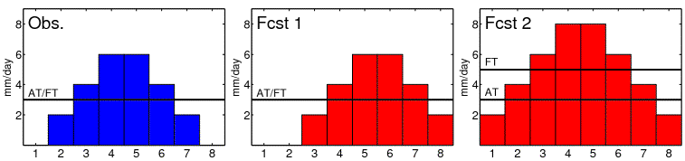
Figure 2: Forecast paradigm of forecasting rainfall amounts for 8 days: Observations (left), first forecast (middle), second forecast (right). The first forecast exhibits a pure shift error of 1 day. The second forecast exhibits a pure bias with an overestimation of 2 mm/day. The selected amplitude threshold (AT) constitutes 3 mm/day. The selected frequency threshold (FT) corresponds to the 50% quantile.

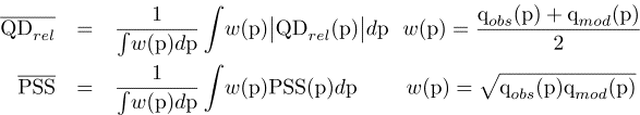
To aggregate the scores over intensities, weighted averages can be computed over quantiles. Thereby, QD_rel is integrated with its absolute value, because individual quantiles with an over- and underestimation can cancel each other out otherwise. The weights w(p) correspond to the arithmetic and the geometric mean for the QD_rel and the PSS, respectively:

A convenient advantage of using quantiles is a stabilization of the sample uncertainty for rare events. Bootstrap confidence intervals for the PSS reveal that the uncertainty usually only slightly increases while moving towards extreme quantiles. Quantile probabilities inherently are not affected by amplitude uncertainties, but their transformation to quantile values, i.e. corresponding amplitudes, suffers from ambiguities. We can achieve a high confidence for the PSS value for a certain quantile, but still hold a low confidence for the quantile estimation. However, since arbitrary amplitudes are not related to the sample distribution, it is sometimes useful only to consider quantiles, corresponding for example to return periods of extreme rainfall events.

An elaborate description of the methodology as well as an application to daily rainfall forecasts of the COSMO1 model over Switzerland can be found in Jenkner et.al. (2008).

A printable pdf version of this web site can be downloaded here.

References:

Gandin, L.S., and A.H. Murphy, 1992: Equitable skill scores for categorical forecasts. Mon. Wea. Rev., 120, 361-370

Jenkner, J., C. Frei, and C. Schwierz, 2008: Quantile-based short-range QPF evaluation over Switzerland. Submitted to Meteorol. Z. download

Mason, I., 1989: Dependence of the critical success index on sample climate and threshold probability. Aust. Met. Mag., 75-81

Stephenson, D.B., 2000: Use of the Odds Ratio for diagnosing forecast skill. Wea. Forecasting, 15, 221-232

Wernli, H., M. Paulat, M. Hagen, and C. Frei, 2008: SAL – a novel quality measure for the verification of quantitative precipitation forecasts. Mon. Wea. Rev., in press

Woodcock, F., 1976: Evaluation of Yes-No forecasts for scientific and administrative purposes. Mon. Wea. Rev., 104, 1209-1214